System Dynamics

A dynamic system is any system that changes with time. This could be a simple mechanical system such as the classical mass-spring-damper system, an electrical circuit, or even a supply chain. The study of system dynamics models these systems and predicts the states of the system (speeds, currents, quantity of goods) at any point in the future.

Below is an example of a simple mass-spring-damper system and the derivation of the system equations. The mass, m, is initially at rest and a force, F, is applied to the mass to excite the system. The ultimate goal of this derivation is to determine the velocity at which the system oscillates and the forces in the mass, spring and damper until the system comes to rest.

There are four types of equations used to derive the system and output equations:

• Node continuity - relates variables of forces or currents (force in equals force out)
• Loop compatibility - relates variables of velocity or displacements (sum of steps in a loop equals the whole)
• Elemental - relates node and loop variables by means of a parameter (F = kx, F is a node variable, k is a loop variable, x is the parameter)
• Energy - defines the amount of energy stored in the element

Node continuity equation:

Loop compatibility equation: v=v

Elemental equations: , ,

Energy equations: , ,

Values of elements: m = 3, b = .2 , k = 1

Initial conditions: , ,

Determine the state variables. These variables are defined to be any energy storage variable (variable in the energy equation). They are the velocity of the system, v, and the force in the spring, F_k.

Use matrix notation. The vector x is defined as the initial values of the state variables v and F_k.

Now that all of the basic equations are written out, start the reduction by solving the loop and node equations for the state variables using the elemental equations. Note that these equations will be differential equations.

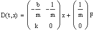
Rewrite the state equations in matrix form. MathCAD was used for solving this problem and the capital D is the differential operator.

Use the Runga-Kutta method to numerically solve the differential equation. Z is a matrix defined to contain the solution to the system for the first 100 seconds, n is a range variable.

The following equations set the solution in the Z matrix to the time and state variables.

, ,

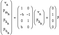
The other variables needed to be solved are the forces in the mass and the damper. Use the elemental equations to solve these and all four variables of interest are defined in the following equation written in matrix form:

Here is a plot of the system response of the four variables: